Distribution-Shift — the hidden reason self-driving cars aren’t safe yet.
- NuronLabs

- Jan 2, 2021
- 5 min read
Have you wondered why self-driving car projections keep getting pushed back from 2018 to 2019 to ‘way in the future’ to ‘may never happen’? While self-driving car prototypes today make for good demos, they are not safe enough to deploy in the real world without substantial human intervention.
One of the main impediments of self-driving car safety is the phenomenon of distribution-shift. This is related to the long-tail problem that’s oft-discussed but is not quite the same. Distribution-shift occurs when the real-world data seen by a model during inference is different from that which it was trained/evaluated on. This is simple to state but is very tricky to manage in practice.
While this is a hard problem to solve perfectly, it is important to address this well in order to bring safe and reliable autonomous vehicles to the market. In this post, we’ll take a closer look at what distribution-shift actually is.
Setup
In this post, we’ll look at distribution-shift in the context of self-driving cars. We will assume that the perception module of the self-driving car learns a discriminative function, e.g. P(Y|X) where the training/test input space, X is an image and the training/test output space Y is a set of class labels (e.g. person, car, bus etc.). In practice X could be a variety of fused or independent input signals such as LiDAR, radar, and multi-view cameras and Y could be detection, segmentation, path planning or control input sequences, etc.
Specifically, we’ll be looking at the differences between the (conditional) probability distributions of X and Y during training and testing to describe the various types of shifts that commonly occur in the real-world.
Types of distribution-shift
There are two main types of distribution-shift that are relevant to self-driving systems, namely, they are domain-shift and label-shift.
Domain-shift

Fig 1. A simplified illustration of the difference in the distribution of visual features between two cities, New York City and Los Angeles. While Los Angeles is known for its Priuses, sports cars, and summer wear, New York is characterized by yellow cabs and formalwear.
Domain-shift, also known as covariate-shift, occurs when the distribution of the testing input domain, Pₜₑₛₜ(X) differs from that of Pₜᵣₐᵢₙ(X). In our context, this refers to the distribution of the visual cues present in the input image. Figure 1. Illustrates a simplified example. In practice, the visual cues are far more complex and can greatly confuse a neural network especially in the long tail. Certain examples also are engineered in the domain to perform adversarial attacks on a neural network. This form of distribution shift is especially hard to detect if the evaluation/validation set is sufficiently close to the training set since the learned distribution Pₜᵣₐᵢₙ(Y|X) correctly classifies the examples that come from Pₜᵣₐᵢₙ(X). It is also important to understand that visual features in the domain vary greatly temporally creating multiple distributional modes. More on this in the examples section below.
Semantic-shift

Fig 2. A simplified illustration of the difference in the distribution of labels at different times of day in the same location. For example, there is usually less vehicular traffic but more pedestrian traffic after lunch as compared to peak-hour.
Another type of distribution shift is semantic-shift, also known as label-shift or prior-shift. This occurs when the distribution of the outputs of the model Pₜₑₛₜ(Y) differ from that of Pₜᵣₐᵢₙ(Y). An example of this would be the difference between pedestrian traffic between peak and non-peak hours in a particular city. Although the appearance of the pedestrians P(X | Y) doesn’t change, their prevalence and behavior do. Failing to account for this might give an unrealistic estimation of the accuracy of the network. As a toy-example, suppose the model sees training data consisting of an equal number of well-separated cars and people. Then the model might perform at a 99.999% accuracy on the validation set, suggesting that the model is ready for real-world deployment. However, if the model sees a crowded street during inference, the previous accuracy estimates may no longer hold true due to label-shift. This could also be problematic if the outputs of the model are used in a downstream task in the system. For example, some AV systems use the output of the perception module for planning and control. This results in a phenomenon known as internal covariate-shift where the intermediate results of each part of the pipeline are no longer well-behaved. A number of non-parametric operations in the model such as non-maximal suppression, object-tracking, refinement/smoothing, pooling, and contextual learning may exaggerate this issue as well.
Distribution-shift in the real world
While the above cases were mostly toy-examples that are easily solved, the real world is much more complex. Let’s take a look at a few examples of distribution-shift in the real world.
1. Location
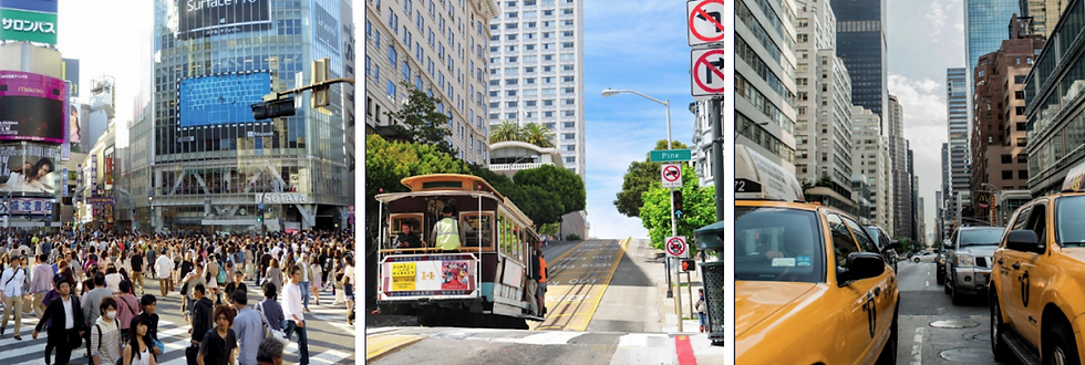
Left: Tokyo, Center: San Francisco, Right: New YorkSome examples of localization induced domain-shift include the difference in preference of vehicle type, differing street signs/markings, types of houses/buildings, people’s dress code, or types of transportation.
2. Time of day

Left: Paris in the morning, Center: Paris at dawn, Right: Paris at night.
The appearance of a location can vary dramatically depending on the time of day. Things like lighting, shadows, and cloud cover patterns can affect this.

Left: New York City during non-peak hours, Right: New York City during peak hours.
As discussed in Fig 2, this also causes label shift due to patterns in human behavior.
3. Seasonal/weather changes

Left: NYC in the Summer, Center: NYC during a rainy day, Right: NYC in the winter.
Seasonal and weather changes also affect domain and semantic shift. This changes behavior patterns, visual appearance, and even road characteristics (inducing a shift in the control domain).
4. Special events

Left: Halloween, Center: Mardi Gras, Right: HoliThe appearance of pedestrians, roads, and their behavior can change dramatically during special events. As the world evolves, these may change quite a bit and models need to adapt quickly.
5. Variations in sensor hardware
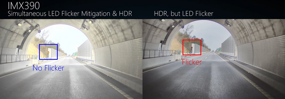
Left: Augmenting the visual domain to better highlight the sign, this results in no flicker, Right: Original image which causes a flicker.
Changes in hardware may introduce subtle domain-shift. While the sensor outputs may look very similar to a human, they may affect the consistency of the neural network. This can sometimes help condition the input better (as in the case above) while hardware settings such as sensor alignment or calibration may also cause errors.
6. Long term non-stationary distributions

Left: Main St. in 2009, Right Main St in 2019.
As time goes on, the structures at a location change. The above example illustrates changes in lanes, buildings, pathways, and signs over a decade. Being able to handle such temporal changes will be an essential component of safe AV systems.
What can we do about this?
The goal of this article is to explain distribution-shift and visually illustrate the complexity of building safe and reliable self-driving cars. While this might initially bring up more questions than answers, the hope is that outlining the complexity serves as a step towards the solution. The first step to solving this is to break down the complexity into manageable sub-problems and building elegant systems that handle these problems. One approach is to brute-force this by building and constantly updating HD maps, training a model with manually added edge case data hoping it learns them adequately, or struggling to incorporate simulated data. While a more elegant approach would be to develop a smarter location-specific closed-loop learning system and continually monitor the safety of a given region. I’d personally bet on the latter.


Comments